2026-04-15
binomial distribution is a very familiar topic for high school kids now a days, it predicts the possibility of number of successes in a trail of bernoulli experiments. this is very useful if parameter \(q\) is well-studied. however in real life, \(q\) is seldomly well-studied, the conjugate problem is more common: given a trail of bernoulli experiments, if the numbers of successes and failures are known, what is the distribution of the underlying probability \(q\)?
baysian theorem offers a practical solution to the question:
decide a prior distribution of \(q\), that is \(p(q)\).
observe the sample \(x\), and hence find the likelihood function \(L(q|x)=p(x|q)\).
update the distribution \(q\), that is \(\displaystyle p(q|x)=\frac{p(x|q)p(q)}{p(x)}\).
depending on the choice of \(p(q)\), the updated distribution \(q\) may or may not has closed form expression. however, for binomial distribution, we can verify that a certain type of prior distribution will maintian its form after the update, that is : \[p(q)\propto q^{x}(1-q)^{y}.\] where \(x\) and \(y\) are expected success and failures. after witnessing the sample \(\alpha, \beta\), the update can be made by \[p(q|\alpha, \beta)\propto \frac{\binom{n}{\alpha}q^{\alpha}(1-q)^{\beta}q^{x}(1-q)^{y}}{\int\binom{n}{\alpha}q^{\alpha}(1-q)^{\beta}p(q)\,\mathop{}\!\text{d}q}.\] notice that the denominator is nothing but a constant, it is shown that the updated believe of \(q\) still has the form of \(q^{x'}(1-q)^{y'}\).
if the type of prior is the same as the updated believe, the prior is referred to as the conjugate prior to the stated distribution.
now let’s standardise the distribution of \(q\). \[\int_{0}^{1}(x, y)q^{x}(1-q)^{y}\,\mathop{}\!\text{d}q=1.\] where \(b(x, y)\) is a function of \(x\) and \(y\in\mathbb N\): \[b(x, y)=\int_{0}^{1}t^{x}(1-t)^{y}\,\mathop{}\!\text{d}t.\] formally, we define the beta function with a shift, that is: \[B(x, y)=b(x-1, y-1)=\int_{0}^{1}t^{x-1}(1-t)^{y-1}\,\mathop{}\!\text{d}t.\] hence the \(\beta\) distribution.
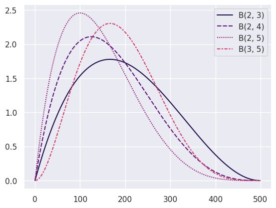
practically, it is widely used in sports games. take, for example, the 3P% of a basketballer. it is generally expected that the average 3P% of a professional player be around 35%, one may well start from a prior believe \[p(r)=\frac{r^{1}(1-r)^{2}}{B(2, 3)}.\] now assume that in a game, the player missed two 3P shot and then mananged to score one, the distribution function would fluctuate as the following, each shot moves the curve a little bit:
it is also noticable that the distribution gets ‘narrower’ as the observation increases, we are more certain when enough observations are made.
additionally, it seems the beta function can be easily extended to \(\mathbb R\), which fractional parameter indicates continuous updating.
think about the function \(B(x, y)\) itself, it’s not difficult to prove the following facts:
\(B(x, y) = B(x, y + 1) + B(x + 1,
y)\),
this comes from the fact that \(t^{x-1}(1-t)^{y}+t^{x}(1-t)^{y-1}=t^{x-1}(1-t)^{y-1}\).
\(B(x, y) = B(y, x)\),
this comes from a substitution \(s=1-t\).
\(\displaystyle B(x + 1, y) =
\frac{x}{y}B(x, y+1)\) and thus \(\displaystyle B(x, y+1)=\frac{y}{x+y}B(x,
y)\),
this comes form an integration by part.
these three properties hint very much about the binomial coefficient, or the combinatoric number. first being the pascal relationship, second being the symmetricity of \(\binom{m+n}{m}\) and \(\binom{m+n}{n}\), the third simply the recursive relationship of binomial coefficient.
when \(x, y\in\mathbb N\), it is straightforward that since \(B(1, 1)=1\), by recursion \[B(x, y)=\frac{1}{\binom{x + y -2}{x - 1}}\frac{1}{x+y-1}\] but the properties do not require integral parameters to withhold, thus, \(\frac{1}{B(x, y)}\) can be thought of the continuous version of binomial coefficient.
naturally, the integration interval \([0, 1]\) and the form of \(t\) and \(1-t\) pair remind one of the trigonometric substitution, let \(t = \sin^{2}\theta\) then \[B(x, y)=2\int_0^{\frac{\pi}{2}}\sin^{2x-1}\theta\cos^{2y-1}\,\mathop{}\!\text{d}\theta.\] a more useful form would be: \[\int_0^{\frac{\pi}{2}}\sin^{n}\theta\cos ^{m}\theta\,\mathop{}\!\text{d}\theta=\frac{1}{2}B\left( \frac{n+1}{2}, \frac{m+1}{2} \right).\] with the recursive property, one would obtain the famous wallis formula.
as the mystery of conjugate prior of binomial distribution is found, it is only natural for one to wonder, what are the conjugate prior of other likelihood functions?
we would establish the fact that \(\beta\) distribution is the prior of bernoulli distribution, thus any counting process of sequence of bernoulli experiments would have \(\beta\) distribution as prior. (meaning geometric and bernoulli distribution)
another well documented conjugate prior of normal distribution is, you guess it, normal distribution.
for poisson distribution, the prior would be something known as the gamma distribution, which is closely related but will be explained in the next post, see you in 2027(?)